Ch.1 Curl, gradient and divergence

Table of Contents

Introduction

Welcome to Chapter 1 of Vector Analysis! This is a self-study guide published to help you study for vector analysis. Vector analysis is a crucially important tool in higher level physics (electromagnetism, fluid dynamics, etc.). If you have previously been doing physics mostly with scalars, it is now time to step it up a notch! Doing physics with vectors will take out a lot of tedious computation, as well as introducing a whole new world of possibilities. To get started, we recommend that you have the following prerequistes:

Should any of the material be unclear to you, please feel free to contact me at: patrick.wang@physics.org

Scalars and vectors, in the context of fields

Let us begin by reviewing the concept of scalar and vector fields. A scalar field is the simplest possible physical field. It is characterised by the property that a point in the field corresponds to a scalar. An example of such a field would be a temperature field. Imagine if we heat a block of metal, and different parts of the metal are heated to different temperatures, we can define a three dimensional basis where a point corresponds to a temperature value. Let us look at another graphical example:

Figure 1: Gravitational Potential Energy as a Scalar Field

Scalar Fields

Suppose we define a 2-dimensional scalar field, where y signifies the distance to the ground, and x is just the horizontal position of an object with mass m. The dotted lines represent the gravitational potential energy of the object, simple enough, it is governed by the equation $V=mgh$, which means for a given value of y, V will stay constant. This is a way of thinking about scalar fields. Imagine “contours”, or in the case above, straight lines, which are imaginary surfaces drawn through all the points in the space which the field has the same value. In the case of potential energy, these field lines are referred to as equipotential lines, or in the case of a temperature field, isothermal surfaces.

Vector Fields

Vector fields are, in some sense, simpler than scalar fields. This idea may be contrary to what you perceive about vectors and rightfully so. Vector calculations are, to put it mildly, quirky, but as we shall see, they are immensely useful in the physical context and arguably make our lives as physicists much easier than scalars would. Similar to scalar fields, vector fields output a vector for a point in space. It goes without saying that both vector and scalar fields can vary in time.

Gradient, derivatives of fields

When fields are time dependent, we can make sense of its behaviour by taking the time derivative, and that is what derivatives really is, a tool to understand the behaviour of something. We can describe variations of position in a similar manner. Suppose we take an example of a scalar field. Imagine a block of metal being heated at various points unevenly, causing the temperature of the block to be different at different points in the block. The heat sources are then removed and we will let the block reach a thermal equilibrium. It is common sense that the temperature of the block will eventually be a constant no matter where you look, as the heat will tend to ‘average it self out’. This is then a time dependent scalar field. What we can do, is take the derivative of temperature with respect to position, to make sense of where the heat is going. But a question arises, for which variable do we take the derivative with respect to? Suppose we are working in 3-dimensional cartesian coordinates, do we operate with respect to \(x\), \(y\) or \(z\)? Here we introduce a concept I would like to refer to as  the Conservation of Vector Quantities. Or in Feynman’s words ‘useful physical laws should not depend on which coordinate system you are in, or even the orientation of said coordinate system.’ To ensure that this is indeed the case, we must choose to write our equations where both sides are either vectors or scalars, not a mixture. Let us refer to the temperature scalar field as \(T\) and then what will \(\pdv{T}{x}\) be? Perhaps you can appreciate the fact that \(\pdv{T}{x}\) is neither a scalar nor a vector, because if we consider the \(y\) and \(z\) axes, surely then \(\partial T\) would then be different! But conveniently, we have three components, \(x\),\(y\), and \(z\). What would happen if we use them as the components of a three-vector?

\[\mqty[\pdv{T}{x}\\ \pdv{T}{y}\\ \pdv{T}{x}]\]

Excercise 1- Proving that this is a vector

Of course it is not generally true that if we have three numbers/variables, they will form a three-vector. But the above quantity is really a vector, a fact which you shall attempt to prove using the fact that if you rotate your coordinate system, the vector transforms itself in a correct way. (Answers below)

Let us first look at an easier version of the proof, one that does not require rotating your coordinate system. Recall the dot product of \(\vec{a}\) and \(\vec{b}\) is a scalar (\(s\)):

\[\vec{a}\cdot\vec{b}=a_xb_x+a_yb_y+a_zb_z=s\]

\(s\), obviously enough, is invariant with different coordinate systems, its just a number. So in otherwords, for every vector \(\vec{a}\), there must exist three numbers such that:

\[a_xb_1+a_yb_2+a_zb_3=s\]

where \(b_{1,2,\text{ and }3}\) corresponds to the three components of some vector \(\vec{b}\)

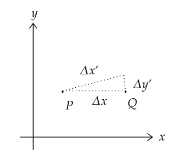
Let’s go back to the temperature field \(T\). Suppose at point \(P\) the temperature of the metal is \(T_P\) and at point \(Q\) separated by a interval \(\Delta \vec{r}\) from \(P\), temperature is \(T_Q\). (\(\vec{r}\) is a vector of three components: \(\Delta x, \Delta y\) and \(\Delta z\), respectively.)The difference in temperature \(\Delta T = T_P – T_Q\). Note that \(\Delta T\) is invariant of the coordinate system, it is a scalar. If we choose a convenient coordinate system, we can write what we have defined simply as: \(T_P=T(x,y,z)\) and \(T_Q=T(x+\Delta x, y+\Delta y, z+\Delta z)\). And using the definition of the partial derivative:

\[\Delta f(x,y,z)=\Delta x\pdv{f}{x}+\Delta y\pdv{f}{y}+\Delta z\pdv{f}{z}\]

(Note that the above definition only works for \(\Delta x,y,\text{ and }z\) approching 0)

we can write:

\[\Delta T=\Delta x\pdv{T}{x}+\Delta y\pdv{T}{y}+\Delta z\pdv{T}{z}\]

The left hand side \(\Delta T\), we know as a fact to be a scalar, where as the right hand side is the sum of three products with \(\Delta x,y,\text{ and }z\), as per our previously proven point at the beginning of this excercise, the components \(\pdv{T}{x},\pdv{T}{y},\pdv{T}{z}\) must form a three-vector. We may express this new vector with the notation \(\nabla T\), it can be read as ‘del’, ‘nabla’ and perhaps more commonly as ‘the gradient of T (grad T)’

If you are still not convinced, perhaps you ought to try it yourself using the method of rotating your axes?

As it happens, this proof will be beneficial in understanding what is about to come, as such, let us go through this together!

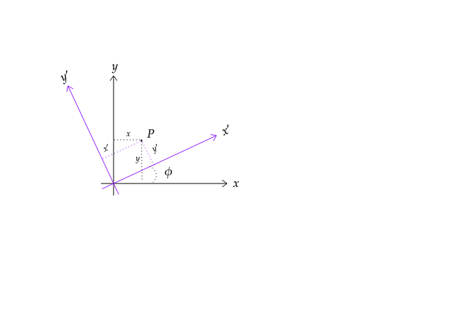
 We shall establish this proof by showing the components of \(\Delta T\) (\(\pdv{T}{x},\pdv{T}{y},\pdv{T}{z}\)) will transform in the exact same way as the components of \(\vec{r}\) do. Let us start by defining a new set of axes, \(x’,y’,z’\). For the sake of ease of visualisation, let us consider the case where \(z=z’\). So the transformation will look something like this:

We can see that the axes are rotated counter-clockwise by an angle \(\phi\). So employing our previous knowledge in linear algebra, we can write the following equations:

\[x’=x\cos \phi + y\sin\phi\]

\[y’=-x\sin \phi+\cos\phi\]

By rearrangement, we can solve for \(x\) and \(y\)

\[x=x’\cos\phi-y’\sin\phi\]

\[y=x’\sin\phi+y’\cos\phi\]

We know that if any pair of numbers transforms in the way the two equations above set to do, they are components of a vector. Let us now establish the quantity \(\Delta T\)

Say we pick a special case, once again, where the line formed by points \(P, Q\) are parallel to the \(x\) axis:

Looking at the above figure, we can deduce:

\[\Delta x’=\Delta x\cos\phi\]

and

\[\Delta y’=-\Delta x\sin\phi\]

And if we were to compute the quantity \(\Delta T\) in the primed system, it would look something like this:

\[\Delta T=\pdv{T}{x’}\Delta x’+\pdv{T}{y’}\Delta y’\]

And because \(\Delta y’\) is negative when \(\Delta x\) is positive, we will find, after substituting what we have deduced above:

\[\Delta T  =\pdv{T}{x’}\Delta x \cos\phi -=\pdv{T}{y’}\Delta x \sin\phi\]

\[\Delta T =\Delta x\left ( \pdv{T}{x’}\cos\phi -\pdv{T}{y’}\sin\phi\right )\]

So now we see that 

\[\pdv{T}{x}=\pdv{T}{x’}\cos\phi-=\pdv{T}{y’}\sin\phi\]

Comparing that to how we obtained \(x\) in the beginning:

\[x=x’\cos\phi-y’\sin\phi\]

We can see its derivative tranforms in the exact same way! Thus, \(\nabla T\) is most certainly a vector. 
So as we previously said, vector quantities should be conserved, then surely \(\nabla\) is a vector? It is a useful mnemonic to think of \(\nabla\) as a vector
\[\mqty[\partial_x\\\partial_y\\\partial_z]\]
but as we shall see, it is a bit deeper than that. 
But what does it all mean? Let us recap.
We have introduced a new property for a scalar valued function called the gradient. It can be found by taking the sum of all of the partial derivatives with respect to all of the variables (however many there may be). The result of said operation will produce a new function, a vector valued function to be specific. 


Geometric Interpretation of \(\nabla T\)

It is helpful to have a mental graphic in mind when thinking about the gradient operator. Below is a Wolfram Notebook figure. You may rotate the view by dragging it with your cursor. 

The yellow mesh in the figure is a parabaloid of the equation:

\[\frac{2}{5}x+\frac{2}{5}y\]

For our purpose, we can consider the parabaloid to be a scalar field. Note that \(z\) is absent from the equation, so we can consider the surface to be a scalar field that for every point \((x,y)\), where \(x,y\in \mathbb{R}\), the field outputs a scalar \(z\).

Let’s now take the gradient of it.

\[\nabla\left (\frac{2}{5}x+\frac{2}{5}y \right )=\left (\partial_x+\partial_y+\partial_z\right ) \left(\frac{2}{5}x+\frac{2}{5}y\right)\]

Which is:

\[\frac{2}{5}x\hat{i}+\frac{2}{5}y\hat{j}+0\hat{k}\]

As we have previously proven, to be a vector.

The resulting vector field are the arrows plotted below the parabaloid. Note that they are pointing away from the origin and lie on the \(x-y\) plane. That is what the gradient operator does! It produces a vector field where the vectors are pointing to the closest steepest ascent, and their magnitude corresponds to the rate at which the field in question is ascending. In the above figure, the magnitude of the vectors are signified by means of colours, the warmer the colour of a vector (i.e. red/orange) the longer it is, and the cooler the colour of a vector (i.e. blue/purple), the shorter it is. Because the parabaloid is symmetric about the \(z\) axis, so it shouldn’t be a surprise that the corresponding gradient vector field points symmetrically away from the \(z\) axis.

Using a programme of your choosing, plot the graph:\(F=\frac{1}{x^2+y^2}\). Note its shape, and then find the corresponding gradient vector field for the graph, hence or otherwise, plot the gradient vector field on the same axes as the surface.

A sample answer may be found here.

Divergence, the derivatives of fields

The divergence of a vector field, as the name suggests, measures the ‘outgoingness’ of the vector field. Let’s go back to the vector field that we derived previously:

\[\vec{F}=\frac{2}{5}x\hat{i}+\frac{2}{5}y\hat{j}+0\hat{k}\],


It is a vector field that points away from the origin uniformly. As you would expect, it has a large value for divergence. Let us evaluate the divergence of said field using the following definition:

\[\div\vec{F}=\partial_xF_x+\partial_yF_y+\partial_zF_z\]

That is, if we consider \(\nabla\) as a vector, it is not, but for our purpose, lets say it is. The divergence of a vector field \(\vec{F}\) is then the ‘dot product’ of it with \(\nabla\). We shall derive this formula from our intuition momentarily, for now, let’s continue with the example.

Following through with the calculation we end up with:

\[\div\vec{F}=\partial_x\frac{2}{5}x+\partial_y\frac{2}{5}y+\partial_z 0=\frac{4}{5}\]

So we now have the divergence of \(\vec F\) to be \(\frac{4}{5}\). Is that correct? One way to visualise the concept of divergence is to put particles in the field, and the vector at the point of the particle will tell where the particle ‘should go’.

I have generated 200 random points over the vector field and directed them to travel in the direction of the nearest vector. As we can see, this is a clearly diverging vector field, so the positive value of \(\frac{4}{5}\) does make sense. This is actually a special case where the divergence value is not dependent on the \(x\) and \(y\) values. It is divergent everywhere on the graph. Let us look at one more example.

Consider the vector field of form:

\[\vec{G}=\mqty[xy\\y^2-x^2\\0]\]

Once again, let us work in 2-dimensions, but keep in mind that all of what we are learning here can be easily extended to 3-dimensions or more.

If we were to plot it, it would look something like this:


Hopefully you can see that the divergence is no longer uniform throughout the field, which in turn, means that our divergence will have \(x\) and \(y\) dependence. It is simple enough to carry out the computation:

\[\div\vec G=y+2y=3y\]

So the divergence of the vector field \(\vec G\) at a point \((x,y)\) is just 3 times the \(y\)-coordinate of said point. Let’s look at an animation of the vector field.


We can start by trying out some values, say we want to know the divergence of the vector field along the line \(y=0\), or the \(x\)-axis. We can look along the axis and notice that there aren’t any discrepancies between the amount of arrows going in and the amount that is coming out. Let’s look out where the points are coming together, roughly around the point \((0,-1)\), which is more a less what we expect as the divergence is -3 at that point, meaning there is more of a converging behaviour. 

The physical significance of the divergence of a vector field is the rate at which “density” exits a given region of space. The definition of the divergence therefore follows naturally by noting that, in the absence of the creation or destruction of matter, the density within a region of space can change only by having it flow into or out of the region. By measuring the net flux of content passing through a surface surrounding the region of space, it is therefore immediately possible to say how the density of the interior has changed. This property is fundamental in physics, where it goes by the name “principle of continuity.”

The formal mathematical definition is:

\[\div\vec F = \lim_{V\rightarrow 0}\frac{\oint_{\partial V}F\cdot dA}{V}\]

It’s quite complex-looking, but we shall come back to this after a few chapters. Though the mathematical definition looks daunting, hopefully the intuition you have developed through looking at the two examples made you comfortable with divergence.

Excercise-

\[\vec H = \mqty[y^3-9y\\x^3-9x\\0]\]

For vector field \(\vec H\), plot either by hand or with a software of your choice, hence, or otherwise, find the general expression for the divergence of \(\vec H\).

An answer has not yet been uploaded.

Curl, the rotation of fields

Curl, similar to divergence is difficult to visualise. It is defined as the circulation of a vector field. Literally how much a vector field ‘spins’. 

The curl operation, like the gradient, will produce a vector. The above figure is an example of rotation, let us look at a 3D example.


Describing Rotation in 3D

The concept of vectors are straightforward enough, a quantity with both a direction and a magnitude associated with it. But what if we want to describe something that is spinning? Some of you may know that an object undergoing circular motion will have a velocity that is aways changing as it goes around the circlular path. We have defined our vectors to be ‘staight’ arrows, not bent arrows. As it turns out, describintg rotation in 3D is really rather simple. To begin describing a system, we first must decide what are the quanlities of the system that we wish to include in our description. For a rotating system, perhaps the direction of rotation (clockwise or counter-clockwise) and the radius of rotation is most important. Ideally, we would want to describe this with one single unique vector. 

As it turns out, it is really quite easy! Rotations are essentially a two dimensional phenomenon. Which means that we have a whole spare dimension to work with!

Let us consider a rotation of radius 1 on the \(x\)-\(y\) plane. We can rotate either clockwise or counter-clockwise (it is also important to define which direction is which, let us suppose we are looking at the plane from \(+z\) direction). For the two cases, we can have two vectors. 

Imagine the rotation being spanned by orthogonal axes that form a plane, and the third axis, the axis of rotation, is what we will use to describe the rotation as a whole. A useful mnemonic to remember which direction the vector that describes the rotation points, is the right hand rule. (This is the exact same as the cross product of two three-vectors.)

Wikipedia- Right Hand Rule

Curl-the formula

The definition is slightly more complicated:

\[\curl \vec{F}=\mqty|\hat{i}& \hat{j}& \hat{k}\\ \partial_x & \partial_y & \partial_z\\ F_x& F_y& F_z |\]

Which is

\[\curl \vec{F}= (\partial_yF_z-\partial_zF_y)\hat i + (\partial_zF_x-\partial_xF_z)\hat j + (\partial_xF_y-\partial_yF_x)\hat k\]

Now that we have drawn the parallel from curl to the cross product (finding an orthogonal vector that describes the rotation), the above formula should really not be surprising at all! 

The curl and divergence, as a useful mnemonic, think of them as the cross and dot products between two vectors respectively. Note that this can only be used as a mnemonic because the \(\nabla\) itself is not actually a vector! A point we shall discuss at length in the next chapter.

Author

  • Patrick

    I am a Chemical Physics student at the University of Edinburgh. I firmly believe that blackboard and chalk should make a comeback. I am die-hard TeX enthusiast, and my favourite fermion is the muon neutrino. You can reach me at patrick@physicswithease.org

Leave a Reply

To write mathematics, simply enclose \(\LaTeX\)in \( \) ext{and}\)\).