
Welcome to the first of a series of articles dedicated to exploring physically interesting differential equations. In most physics students’ minds unfortunately, differential equations are just labeled as ‘that maths tool I might need one day’, resulting in a general attitude of indifference and perhaps mild annoyance. I hope through this series of articles on differential equations modelling physically interesting systems, and extensive use of visulisations, that you genuinely do find differential equations absolutely fascinating. It is crucial that you see beyond the façade that is fancy nomenclature.
Perhaps it is appropriate for us to start with a rudimentary but nevertheless interesting system, the Newton Pendulum. We start with a couple previously known equations that are not differential equations:
\[\vec{F}=m\vec{a}\]
\[\vec{\alpha}=\frac{\vec{a}}{L}=L\frac{d^2\theta}{dt^2}\]
The first equation, needs no introduction, is the Newton’s Second Law. Where as the second equation, is an expression for angular acceleration (\(\alpha\)), which can also be written as the second time derivative of \(\theta\), the angle the pendulum’s string makes with the vertical. Multiplying m to the angular acceleration will yield the following:
\[mL\dv[2]{\theta}{t}=mg\sin\theta\]
You will note that I replaced the right hand side with the vertical component of acceleration due to gravity. You will also note that m cancels on both sides, which is concordant with physical observations, the mass of a pendulum has no effect on the period of its oscillations. Hopefully you will have realised the fact that we now have an ordinary differential equation of the second order, though the sine on the RHS makes this excruciatinglly non-linear. With no appararent substitutions, we shall attempt to solve this graphically.
We can start by rewriting the differential equation as two coupled-first order differential equations, let us define some variable \(\eta\)
\[\eta= \dv{\theta}{t} \]
\[\dv{\eta}{t}=\dv[2]{\theta}{t}\]
We can now think about this as a first-order problem that spans the 2 dimensional plane \([\theta,\eta]\), where the solution to the DE are the trajectories \([\theta (t),\eta (t)]\). In addition, at any point on the plane, the trajectory must be tangent to the vector \([\dv{\vec{\theta}}{t}, \dv{\vec{\eta}}{t} ]\). We now have expressions for a 2-dimensional vector field. We can either choose to draw this by hand, or use a mathematical programme (I am using Wolfram Mathematica for this example).
In[]: StreamDensityPlot[{\[Eta], -Sin[\[Theta]]}, {\[Theta], -\[Pi], \
\[Pi]}, {\[Eta], -5, 5}, ColorFunction -> Hue,
 PlotLegends -> Automatic, FrameLabel -> {\[Theta], \[Eta]}]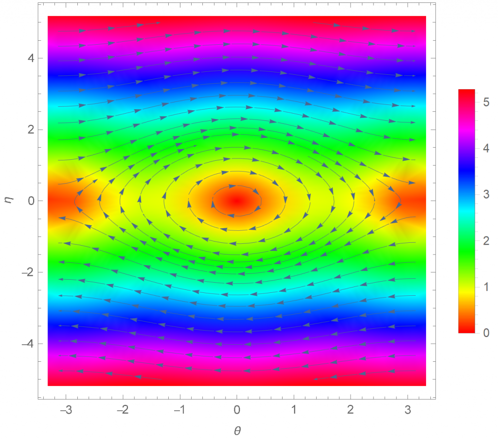
The picture is quite pretty, but let us try and make sense of it. The vectors point towards the direction of motion, imagine if you are standing on a point in the graph, your motion will follow the direction of the vector, as if you are flowing in a river. The x-axis represents \(\theta\) and the y-axis represents \(\dv{\theta}{t}\), or \(\omega\). Let us pick a point and see if the plot is how we would expect a pendulum to behave. Take a small \(\theta\), near the centre of the plot, we would expect an oscillation of a small amplitude, and that is exactly what we get! If you imagine yourself standing in the middle of the plot, and follow the arrow, you end up going back and forth with a small angular displacement. Furthermore, I have included the option a colour map to the plot, where red signifies 0. See if it makes sense to you that there are three small red regions in the plot. It makes sense for the velocity at the maximum height of the amplitude to be 0, hence the red regions on the two ends of the plot, in addition to the ‘no oscillation at all’ red region in the centre when \(\theta\) tends to 0.
\begin{document}
\[E=mc^2\]
\end{document}
As some of you have rightfully pointed out that \(\frac{d}{dt}\) is indeed not the correct way of writing the differential operator. I have since loaded the physics package, and so this should look better :\(\dv{t}\).